Signal Processing toolkit

Links: Github | PyPi - project

Installation: pip install spkit

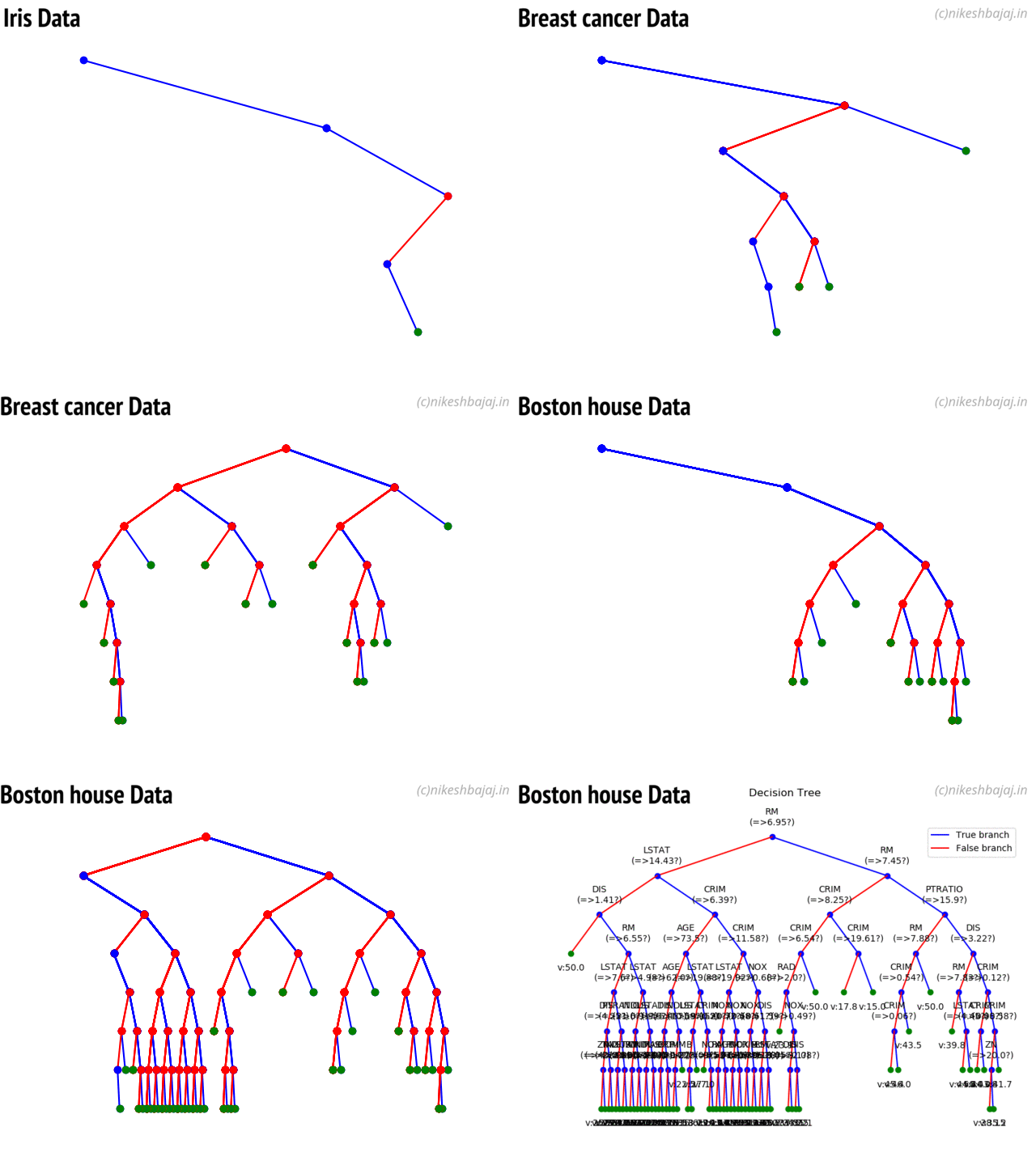
Updates:: Decision Tree

---

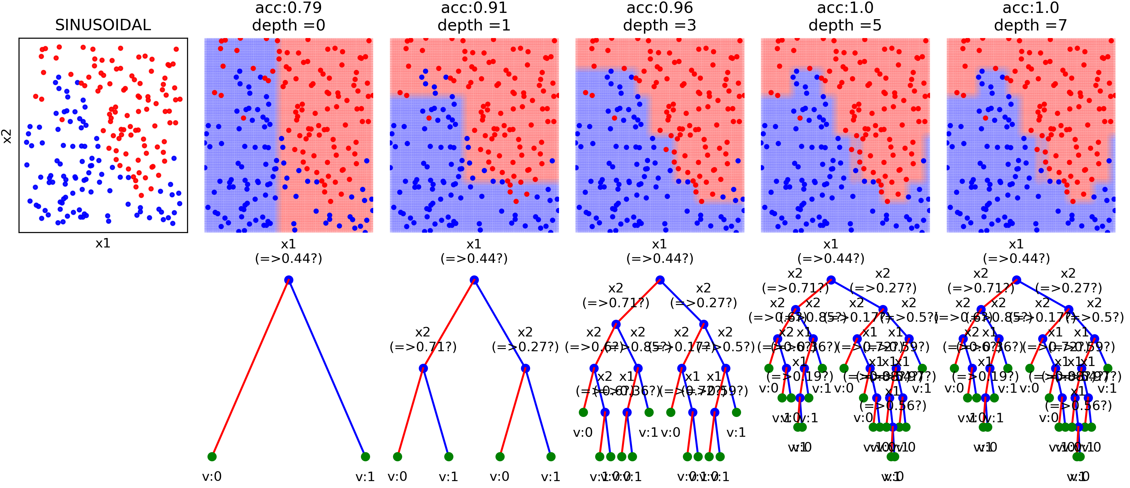
Table of contents

• Installation
• Signal Processing & ML function list
• Examples
  • Information Theory
  • Machine Learning -Logistic Regression -Naive Bayes -Decision Trees
  • ICA
  • LFSR

---

Installation

Requirement: numpy, matplotlib, scipy.stats, scikit-learn

with pip

pip install spkit

Build from the source

Download the repository or clone it with git, after cd in directory build it from source with

python setup.py install

Functions list

Signal Processing Techniques

Information Theory functions for real valued signals * Entropy : Shannon entropy, Rényi entropy of order α, Collision entropy * Joint entropy * Conditional entropy * Mutual Information * Cross entropy * Kullback–Leibler divergence * Computation of optimal bin size for histogram using FD-rule * Plot histogram with optimal bin size

Matrix Decomposition * SVD * ICA using InfoMax, Extended-InfoMax, FastICA & Picard

Linear Feedback Shift Register * pylfsr

Continuase Wavelet Transform and other functions comming soon..

Machine Learning models - with visualizations

• Logistic Regression
• Naive Bayes
• Decision Trees
• DeepNet (to be updated)

Examples

Information Theory

View in notebook

import numpy as np
import matplotlib.pyplot as plt
import spkit as sp

x = np.random.rand(10000)
y = np.random.randn(10000)

#Shannan entropy
H_x= sp.entropy(x,alpha=1)
H_y= sp.entropy(y,alpha=1)

#Rényi entropy
Hr_x= sp.entropy(x,alpha=2)
Hr_y= sp.entropy(y,alpha=2)

H_xy= sp.entropy_joint(x,y)

H_x1y= sp.entropy_cond(x,y)
H_y1x= sp.entropy_cond(y,x)

I_xy = sp.mutual_Info(x,y)

H_xy_cross= sp.entropy_cross(x,y)

D_xy= sp.entropy_kld(x,y)


print('Shannan entropy')
print('Entropy of x: H(x) = ',H_x)
print('Entropy of y: H(y) = ',H_y)
print('-')
print('Rényi entropy')
print('Entropy of x: H(x) = ',Hr_x)
print('Entropy of y: H(y) = ',Hr_y)
print('-')
print('Mutual Information I(x,y) = ',I_xy)
print('Joint Entropy H(x,y) = ',H_xy)
print('Conditional Entropy of : H(x|y) = ',H_x1y)
print('Conditional Entropy of : H(y|x) = ',H_y1x)
print('-')
print('Cross Entropy of : H(x,y) = :',H_xy_cross)
print('Kullback–Leibler divergence : Dkl(x,y) = :',D_xy)



plt.figure(figsize=(12,5))
plt.subplot(121)
sp.HistPlot(x,show=False)

plt.subplot(122)
sp.HistPlot(y,show=False)
plt.show()

ICA

View in notebook

from spkit import ICA
from spkit.data import load_data
X,ch_names = load_data.eegSample()

x = X[128*10:128*12,:]
t = np.arange(x.shape[0])/128.0

ica = ICA(n_components=14,method='fastica')
ica.fit(x.T)
s1 = ica.transform(x.T)

ica = ICA(n_components=14,method='infomax')
ica.fit(x.T)
s2 = ica.transform(x.T)

ica = ICA(n_components=14,method='picard')
ica.fit(x.T)
s3 = ica.transform(x.T)

ica = ICA(n_components=14,method='extended-infomax')
ica.fit(x.T)
s4 = ica.transform(x.T)

Machine Learning

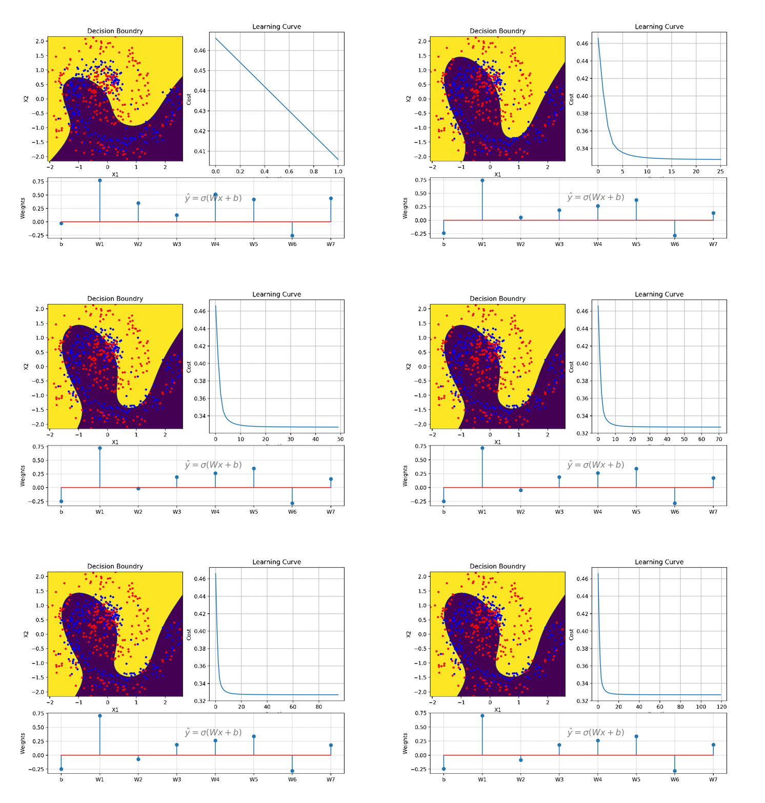
Logistic Regression - View in notebook

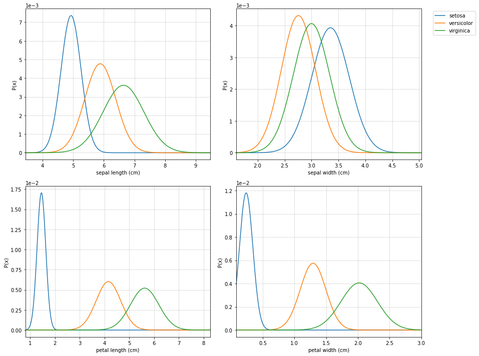
Naive Bayes - View in notebook

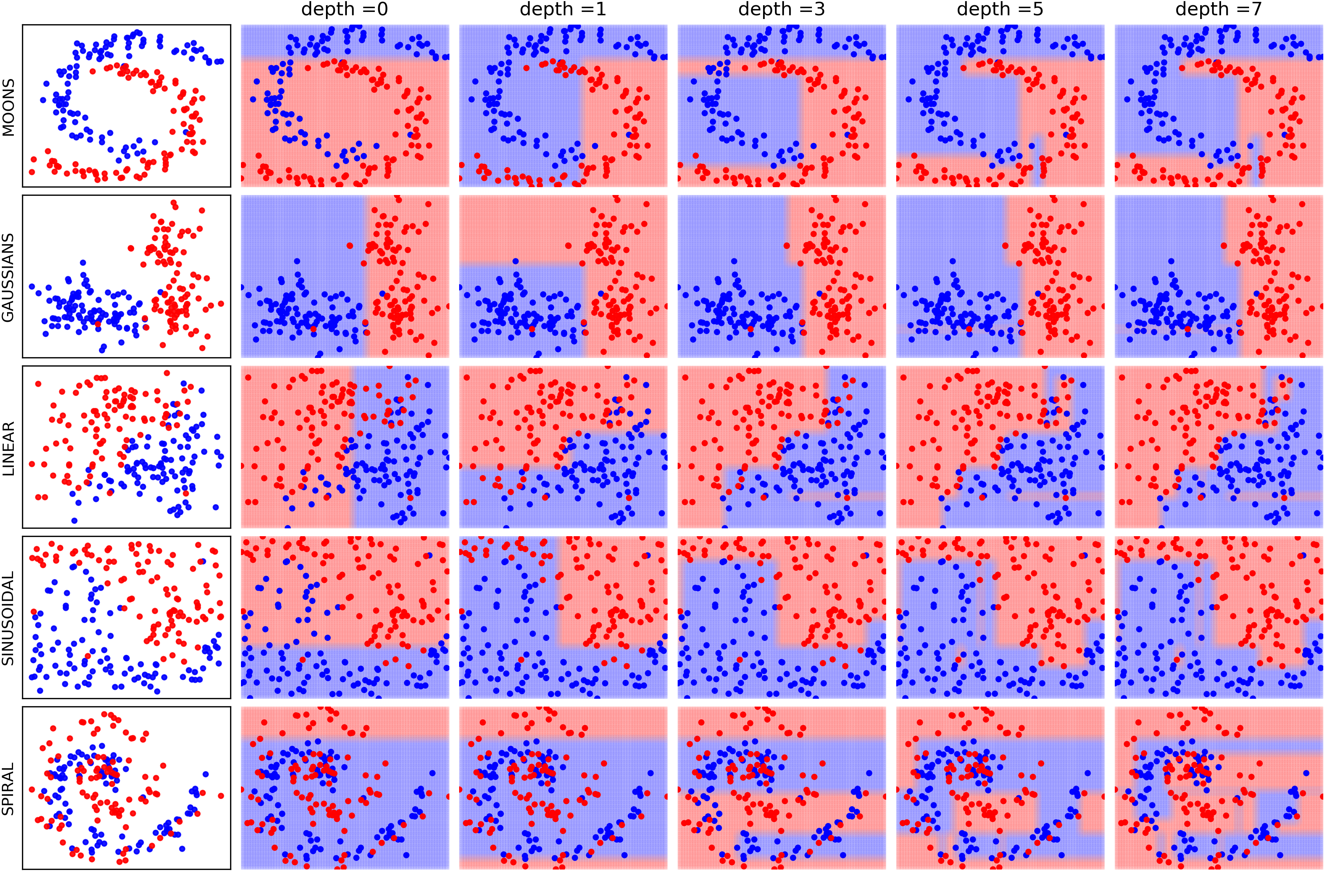
[Decision Trees]

(https://nbviewer.jupyter.org/github/Nikeshbajaj/spkit/blob/master/notebooks/2.3_Tree_Example_Classification_and_Regression.ipynb) - View in notebook

This implimentation also works with Catogorical features, without need to change them into float or interger type

[source code] | [jupyter-notebook]

Plottng tree while training

**view in repository **

LFSR

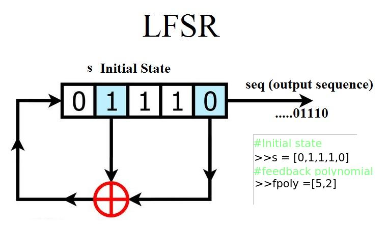
import numpy as np
from spkit.pylfsr import LFSR
## Example 1  ## 5 bit LFSR with x^5 + x^2 + 1
L = LFSR()
L.info()
L.next()
L.runKCycle(10)
L.runFullCycle()
L.info()
tempseq = L.runKCycle(10000)    # generate 10000 bits from current state

---

Contacts:

• Nikesh Bajaj
• http://nikeshbajaj.in
• n.bajaj@qmul.ac.uk
• bajaj.nikkey@gmail.com

PhD Student: Queen Mary University of London & University of Genoa

---